Many problems in real life can be represented as optimization problems that are subject to various constraints. How far can I go without stopping at the gas station if I expect to drive 60% on the highway and 40% in the city? What’s the most enjoyment I can get with $10 of chocolate bars, given that I want at least one Butterfinger bar but like Snickers twice as much? How can I achieve the best GPA given my current grades in the classes, each class’s grading system, and that I only have 2 more days to study for finals?
The simplex method is an algorithm for finding a maximal function value given a set of constraints. We’ll start with a non-trivial example that shows why we need a rigorous method to solve this problem, then move on to a simple example that illustrates most of the main parts of the simplex method. You’ll learn when to use it, you can check out my cheatsheet, and you can review my code on github!
To look at a concrete example of this kind of non-trivial problem, suppose you are CEO of an agricultural company that grows 3 types of crops – wheat, corn, and alfalfa. Since you’re a pragmatic and conscientious farmer, you rotate crops to prevent disease and increase yield. This year, based on the crop’s locations, some soils & topologies are nearly perfect for a given crop (and adding water or fertilizer will actually reduce yields) while other soils & topologies need assistance to produce maximum yield.
Your scientists have determined, for each crop in its planned location, the change in yield for each additional $1000 spent on irrigation, fertilization, herbicide application, and pesticide application; these values are described in Table 1 below. Your job is to determine the cheapest method to satisfy your customer’s demands of 80k pounds of wheat, 50k pounds of corn, and 100k pounds of alfalfa.
| Action | Wheat | Corn | Alfalfa |
|---|---|---|---|
| Base production (yield while taking no action) | 17000 | 50000 | 1000 |
| Irrigate | +400 | -100 | +500 |
| Fertilize | -300 | +500 | +100 |
| Apply weed killer | -500 | -200 | +200 |
| Apply pesticide | +500 | +300 | +400 |
Table 1: The effect on yield in pounds, per $1000 of spending on the given action
One method of solving this problem is by trial and error, but this is very likely to produce a plan that is not the cheapest. For example, you could spend $150,000 on irrigation, $0 on fertilizer, $0 on weed killer, and $60,000 on pesticide. This would result in the following yields:
| Wheat |
17000 + 150 * 400 - 0 * 300 - 0 * 500 + 60 * 50 = 80000 |
|---|---|
| Corn |
50000 - 150 * 100 + 0 * 500 - 0 * 200 + 60 * 300 = 53000 |
| Alfalfa |
1000 + 150 * 500 + 0 * 100 + 0 * 200 + 60 * 400 = 100000 |
Table 2: Example yields given trial & error values for each possible action.
With this spending, you’re able to produce exactly the amount of wheat and alfalfa that you need, though you overproduce corn. However, how can we verify that this is an optimal (cheapest) solution to producing enough of each crop?
Graphical Analysis
To develop the simplex method, we’ll look at a simpler example that can be easily plotted, for which the correct answer is intuitive and easily verified.
Suppose you’re in charge of a bake sale. You’ve decided to sell two products, cupcakes and pie slices. Cupcakes sell for $1, and mini pies sell for $2; note that this example does not reflect my personal opinion of the relative deliciousness of cupcakes and mini pies. You’ve determined that you have enough ingredients to make 120 cupcakes, or 40 mini pies, but you only have enough oven time to bake 50 total items. You know that whatever you make will sell out. Your goal is to maximize the revenue, so how many of each product should you make?
We can write out our optimization like this, where X is the number of cupcakes we can make and Y is the number of mini pies we can make:
0 <= X <= 120
0 <= Y <= 40
X + Y <= 50

We want to maximize our total revenue R:
1 * X + 2 * Y = R
Here’s the graphical representation of the inequalities:
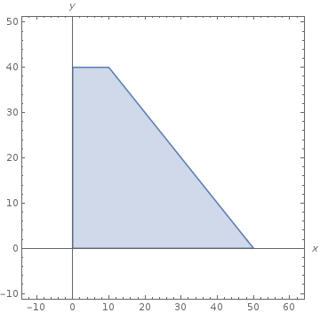
Plot of x>=0, y>=0, x<=120, y<=40, and x+y<=50
This shows the intersection of the regions defined by various inequalities: X is between 0 & 120, Y is between 0 & 40, and X + Y is less than 50. So it’s pretty obvious that the optimal solution must be somewhere in this region. But how do we know what’s the optimal solution?
This problem is simple enough to be solved graphically. For any constant R, X + 2Y = R defines a line. For example, here are the lines for X + 2Y = 10, X + 2Y = 60, and X + 2Y = 100 overlaid on the region.
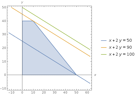
3 possible objective functions overlaying the feasible region
You can see that the line for R = 100 does not intersect the region, the line for R = 90 intersects the region at exactly one point, and the line for R = 50 intersects the region in the range X = [0, 50].
So, we can see that this region is convex. We can see that if R = 90 + epsilon, the line X + 2Y will not intersect the region. Therefore 90 is the maximum value of X + 2Y that intersects the region and it occurs at (X, Y) = (10, 40). This is exactly what we would expect given our constraints – to maximize our revenue, sell as many $2 mini pies as possible, then sell as many $1 cupcakes as possible.
Here are the important points to note in this example:
- The inequalities define a region in space, called the feasible region
- There is at least one solution, because the region is non-empty
- The objective function (what we’re trying to minimize) is a line
- The solution to the optimization problem occurs at a vertex of the feasible region
In fact, it sort of makes sense that the solution is at a vertex: a given inequality must have its minimum or maximum value along the boundary that it defines. This is the key insight that leads to the simplex algorithm: we will find some vertex of the feasible region, then travel along an edge to another vertex with a non-smaller value for the objective function, and so on, until we cannot find any vertices that have a larger value for the objective function.
Simplex Algorithm
I’m not going to cover things like the setup and terminology in detail. There are excellent explanations in (for example) Introduction to Algorithms, and you can also review my reference sheet. I just want to cover how the simplex algorithm works. But, to make this a pretty much standalone article, I’ll cover those things briefly.
Also, for consistency and without losing generality, I’m going to change most of the variable names to xi, where i is the index of the variable.
Terms
Standard form
This is basically:
- Writing the objective function as a maximization objective in a first degree polynomial
- Adding inequalities for all the variables so they are greater than or equal to zero
- Writing the rest of the inequalities as less-than-or-equal-tos
The bake sale example would be written in standard form like this:
Maximize:
1*x1 + 2*x2 = z

Subject to:
x1 <= 120
x2 <= 40
x1 + x2 <= 50
x1, x2 >= 0
Slack form
The slack form converts the standard form into an equivalent a system of equalities and inequalities. This makes the simplex algorithm easier for a computer to process, because we’re dealing primarily with equalities.
To perform the conversion, we’ll transform the system of inequalities so that all the inequalities are transformed into non-negativity inequalities. This is done by introducing new variables.
For example:
x1 <= 40
converts to:
x3 = 40 - x1
x3 >= 0
Here’s the bake sale example in slack form:
Maximize:
1*x1 + 2*x2 = z

Subject to:
x3 = 120 - x1
x4 = 40 - x2
x5 = 50 - x1 - x2
x1, x2, x3, x4, x5 >= 0
Basic/nonbasic variables
In the slack form, the basic variables on on the left side, and the non-basic variables are on the right side.
Feasible solution
A feasible solution is a setting of the variables that satisfies all the constraints. Basically it’s a set of variable values that appear inside the shaded area of the graph.
Feasible region
The set of feasible solutions. Basically it’s the shaded area of the graph.
Operations
There are some “primitive” (ha!) operations that we’ll use in the algorithm.
Basic solution
In the slack form, set all the non-basic variables to zero. This is a simple procedure for generating values of the basic variables, because the basic variables will take on the values of the constants from each equality. The basic solution for the slack form above is:
x1 = 0
x2 = 0
x3 = 120
x4 = 40
x5 = 50
Given these variable values, the objective function will have the value 0.
1*0 + 2*0 = 0
Pivot
A pivot swaps a basic for a non-basic variable by solving for the non-basic variable, then substituting the resulting equation into every other equation. This produces an equivalent system of equations because all we’re doing is shuffling things around.
For example, if we wanted to pivot x2 & x4, we would solve for x2 in the first equation and find that:
x2 = 40 - x4
Then we could substitute this into all other equations:
Maximize:
x1 + 2*(40 - x4) = z

Subject to:
x3 = 120 - x1
x2 = 40 - x4
x5 = 50 - x1 - (40 - x4)
   = 10 - x1 + x4
x1, x2, x3, x4, x5 >= 0
We can get a basic solution for this system by setting x1 = x4 = 0:
x1 = 0
x2 = 40
x3 = 120
x4 = 0
x5 = 10
And if we plug these values into the resulting objective function, we see that z has the value 80. This is comforting because previously z = 0, and the simplex algorithm is supposed to incrementally find non-smaller values for the objective function, which it has. An increasing value for the objective function probably means we’re doing the right things.
Pivot choice
I glossed over a step above by choosing to pivot x2 & x4. What we’re trying to do with the simplex algorithm is gradually increase the value of the objective function until it can’t be increased any more. We previously saw that by pivoting x2 & x4, the value of the objective function increased from 0 to 80. It’s possible that a choice could cause the objective function value to remain constant, or even decrease. How do we know which variables to choose so that a pivot produces a basic solution that increases the objective function value? Let’s review the original slack form:
Maximize:
1) 1*x1 + 2*x2 = z

Subject to:
2) x3 = 120 - x1
3) x4 = 40 - x2
4) x5 = 50 - x1 - x2
5) x1, x2, x3, x4, x5 >= 0
Recall that all variables xi must be non-negative due to the non-negativity constraints in line 5. Looking at the original objective function x1 + 2*x2 = z in line 1, we can increase z by increasing x1 or x2, because x1 & x2 have positive cofficients.
Let’s choose x2. How far can it be increased without violating the constraints? Well, it can be increased to 40 in line 3, because any value > 40 would cause x4 to become negative. It can be increased to 50 in line 4, because if we set x1 to the minimum value (0), increasing x2 > 50 would cause x5 to become negative. We’ll choose to pivot around the minimum of these possible increases to guarantee that we don’t violate any constraints, therefore we choose to pivot around x4 in line 3.
As we previously saw, this produces the new set of equations:
Maximize:
1) x1 + 80 - x4 = z

Subject to:
2) x3 = 120 - x1
3) x2 = 40 - x4
4) x5 = 10 - x1 + x4
5) x1, x2, x3, x4, x5 >= 0
It’s worth mentioning a final note about this pivot choice. The initial basic solution had (x1, x2) = (0, 0), which is a vertex of the feasible region in the graph. After the first pivot, basic solution for the system above has (x1, x2) = (0, 40). This is also a vertex of the feasible region in the graph above. So we’ve used the simplex method to move from one vertex to another, increasing the value of the objective function along the way! Neat.
Completing the example
Now we continue with similar reasoning. In the objective function, since x4 must be non-negative and it has a negative coefficient, any valid value for x4 must cause z to remain constant or decrease. Any valid value for x1 must cause z to remain constant or increase. Therefore we’ll choose to pivot around x1.
From line 2, we see that x1 can increase to 120 without violating the non-negativity constraint on x3. From line 4, we see that x1 can increase to 10 without violating the non-negativity constraint on x5. So, choosing the minimum of these values, we will choose to pivot around x5 in line 4:
x1 = 10 - x5 + x4
Which produces the following system:
Maximize:
1) (10 - x5 + x4) + 80 - x4 = z
   90 - x5 = z

Subject to:
2) x3 = 120 - (10 - x5 + x4)
      = 110 + x5 - x4
3) x2 = 40 - x4
4) x1 = 10 - x5 + x4
5) x1, x2, x3, x4, x5 >= 0
The basic solution for this system is found by setting x4 = x5 = 0:
x1 = 10
x2 = 40
x3 = 110
x4 = 0
x5 = 0
And the value of the objective function given this basic solution is z = 90. Since all the coefficients in the objective function are non-positive, we know that the objective function value cannot be increased any further without violating the non-negativity constraints. Therefore this is the maximal value of the objective function and we are done.
Important note: we found the same solution graphically and algorithmically (secret sigh of relief)! We matched both the maximum value of the objective function, and the point where it occurs. So we got that going for us, which is nice.
Conclusion
So I hope that’s a simple explanation of the simplex method. In a nutshell, after converting the problem into slack form, we iteratively perform these operations:
- Find a basic solution
- Compute the objective function value using basic solution values
- Choose pivot variables – stop when all coefficients of the objective function are negative
- Perform a pivot
When to use it
This technique is surprisingly powerful. It allows you to find an optimal value of a linear function given an arbitrary number of linear constraints over an arbitrary number of variables. Situations where this might be valuable include:
- Diet management – find the cheapest combinations of foods that will satisfy your nutritional requirements (warning: may produce unpalatable diets!)
- Crew scheduling – find minimum cost for airline crews subject to ensuring every flight has a crew, crews can’t work more than X hours/day, crews must have minimum time between flights, etc.
- Transportation – find the cheapest route for a good from one city to another while accounting for driver compensation, depreciation of value of goods, toll roads, etc
Besides its applicability to only linear relationships, use of this technique is truly limited only by your imagination! Perhaps a better way to determine when to use this technique is by asking some questions:
- Is it a minimization or maximization problem (yes/no)?
- Can the relationships between the variables be expressed linearly (yes/no)?
If the answer to these two questions is yes, the problem can be formulated as a linear program and the simplex method can be used.
I’ve posted a slightly modified version of my own simplex algorithm code as a gist on github, written while I took an Advanced Algorithms and Complexity course on Coursera. It was originally written to solve the diet problem, but is easily generalized to any linear problem. Feel free to comment here or directly on the gist if you have any questions!
Other very important points
I ignored many very important, perhaps even fundamental, aspects of linear programming and the simplex method, including:
- How can we determine if there are any feasible solutions to a given set of inequalities? (answer: there is an initialization procedure that I didn’t discuss that can tell us whether there are any feasible solutions)
- What if some constraints are equalities rather than inequalities? (answer: replace with 2 inequalities; replace x1 = x2 with x1 <= x2 and x1 >= x2).
- How do we handle a minimization problem instead of a maximization problem? (answer: min(z) == max(-z))
- Does the algorithm work if the initial basic solution is not a feasible solution? (answer: no – the initialization procedure can find a feasible solution if the initial basic solution is not feasible)
- How do we handle constraints that are greater-than-or-equal-to, instead of less-than-or-equal-to? (answer: x1 >= x2 is equivalent to -x1 <= -x2)